How To Use - Use Case Overview

Following is a tutorial to help the use of Mimer for visualization and knowledge discovery. This tutorial offers a step-by-step guide a user should be able to replicate to reach the same results

Data

This tutorial uses the following dataset:
 tdata1
Which contains the non-dominated solutions from one run of the RE3-5-4 problem from the RE problem suite[1]. RE3-5-4 is a three objective problem (min_f0, min_f1, min_f2) with five decision variables (x0 - x4).
The dataset contains 1894 solutions, and the structure of the objective space show three clear clusters.

Loading a Multi-Objective Optimization Problem (MOOP) Dataset

This tutorial uses the tdata1 dataset.
There are two ways to load a dataset:

1. by clicking the "Load Dataset" button
2. by dragging the csv file into the page

Mimer expects a "flat" csv file with the first row defining the headers, and will do its best to figure out the delimiter, however, a safe bet is to use a "," or ";".

Visualization of MOOP Dataset

Mimer offers several methods for visualizing data:

1. 2d and 3d scatter plots
2. Parallel coordinate plots (PCP)
3. RadViz[2]
4. t-SNE[3]
5. UMAP[4] (Currently under development)

tdata1 is a 3d objective space, so it can be visualized using a 3d scatterplot.
To open a new plot, click on the dataset in the list of loaded dataset, and then choose the plot type you want.
All plots in Mimer are interactive, a 3d scatterplot can be rotated and panned by dragging with the mouse.

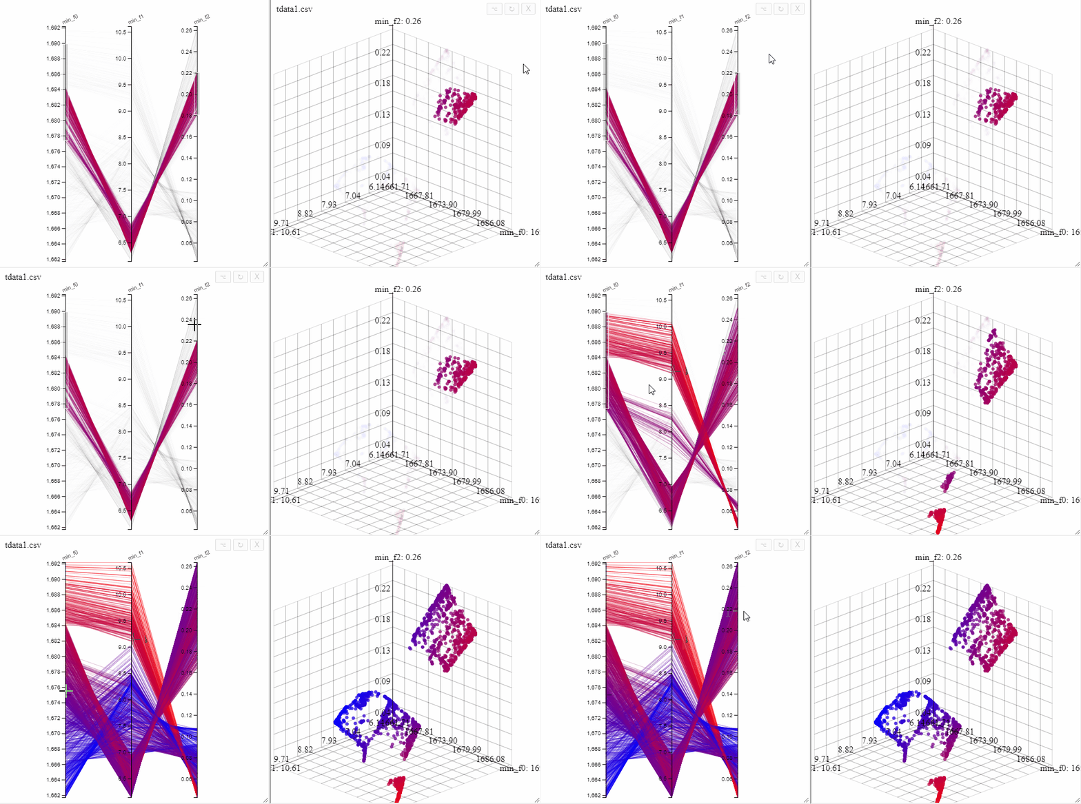
All plots opened on the same dataset are linked, opening both a 3d scatterplot and a parallel coordinate plot allows simultaneous filtering of solutions in both plots.

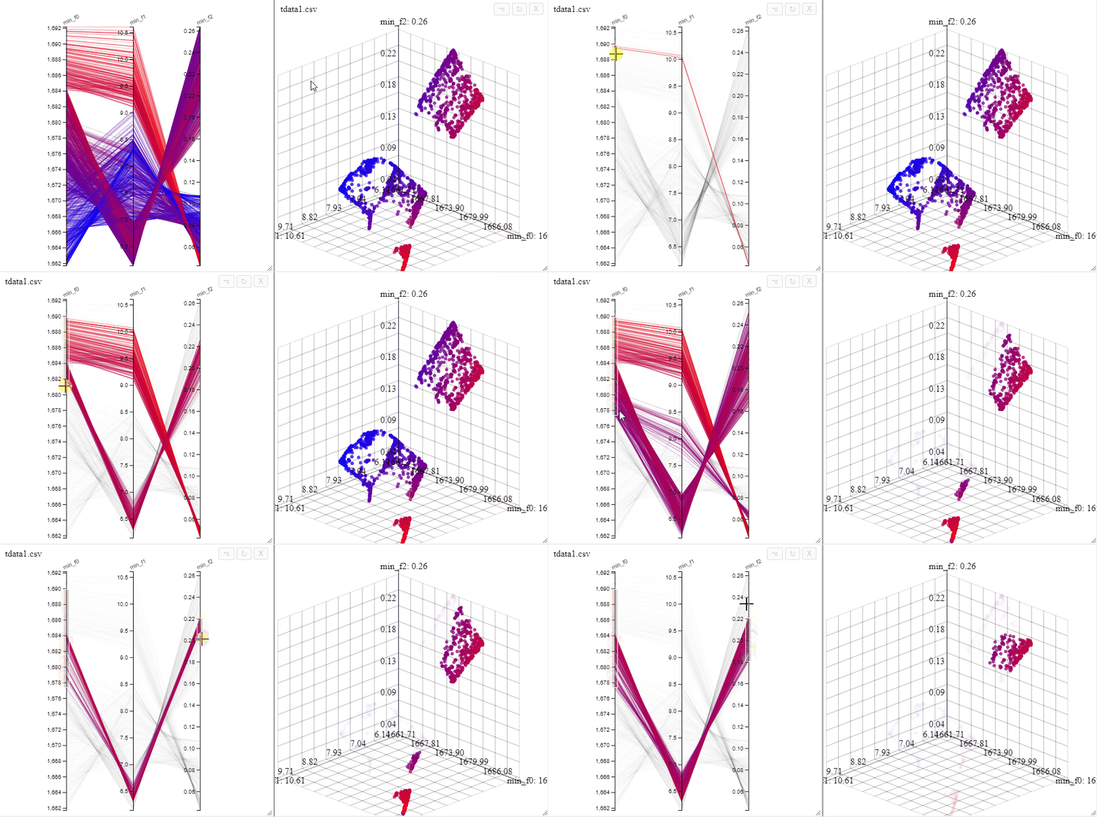
A filter can also be removed by clicking on the same axis in the parallel coordinate plot.

Preference Elicitation

There are three ways for selecting solutions to articulate the DM's preferences:

1. Lasso-based selection (Appropriate for 2d plots, like 2d scatterplot and RadViz)
2. Slider-based selection (Appropriate for PCP)
3. Reference point-based selection (Currently under development)

Solutions can be highlighted by lassoing them with the mouse.

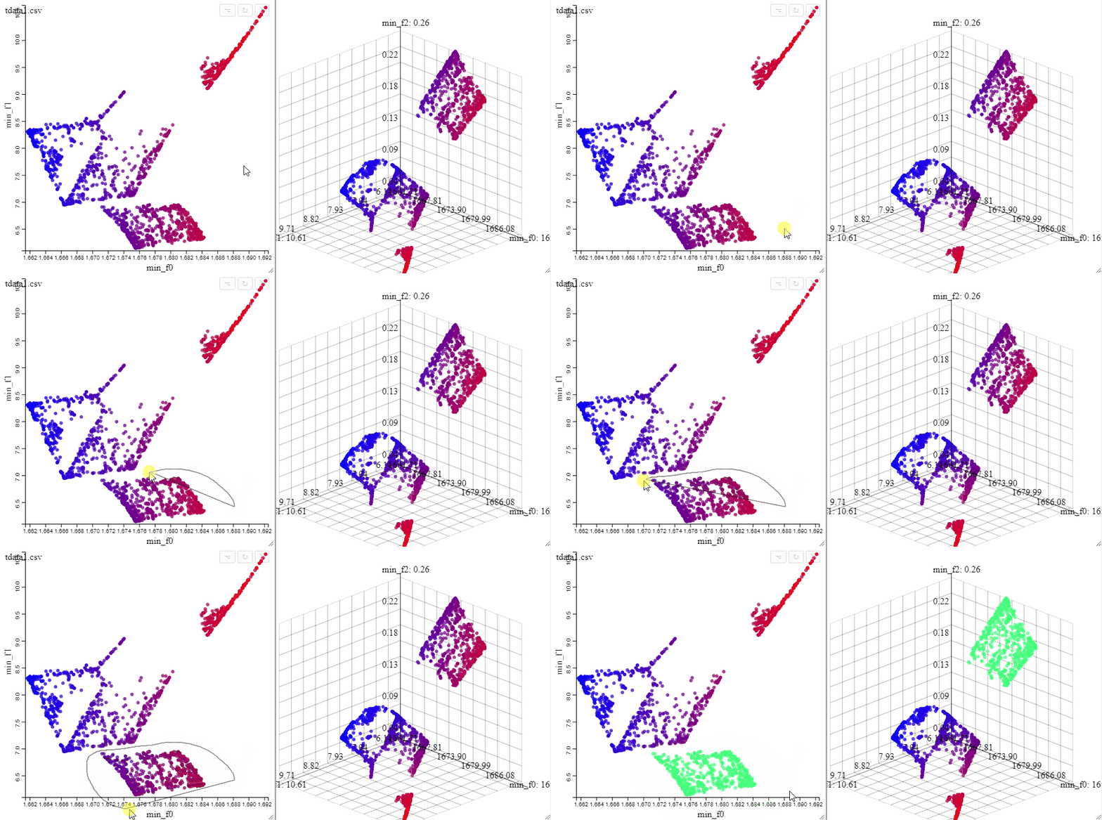
Several selections can be made at the same time by changing the color.

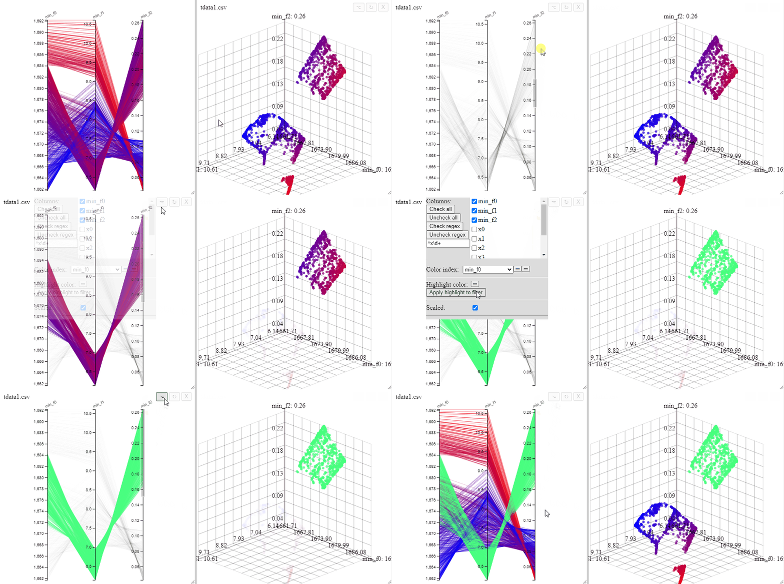
Filters made in a PCP can be turned into a selection.

Interactive Knowledge Discovery

There are two ways of extracting explicit knowledge in the form of decision rules from the selected solutions:

1. Flexible Pattern mining (FPM)[5]
2. Simulation based Innovization (SBI)[6] (Currently under development)

To generate FPM rules, a 'selected' and an 'unselected' set of solutions need to defined. This is done by choosing a color used to select solutions in the plots.
First open the FPM options pane and select the dataset and 'selected' and 'unselected' sets.

It is also possible to use one selection for the 'selected' set and one for the 'unselected' set, while omitting the remaining solutions.

The next step is to define the variables you want to include. They can be chosen individually, or (if there are many variables) they can be chosen use regular expressions.

The final step is to define the parameters for FPM and run the procedure. 'Min. Sig.' refers to the minimum significance that a rule is allowed to take, 'Max. Levels' refers to the maximum number of rule-interaction levels to generate rules for, and 'Min. interaction sig.' refers to the minimum significance a rule-interaction is allowed to take. For some datasets, the FPM procedure may be very time consuming, increasing the minimum significance will generate only the most significant rules, which will be faster. But the default is a good place to start.
And finally the name the generated rule set can be determined, and after clicking the button 'Run FPM', the rules will be generated and added to the list of rulesets.

Interactive Knowledge Visualization

To visualize a ruleset, click on it in the list of rulesets and then open the FPM graph plot.

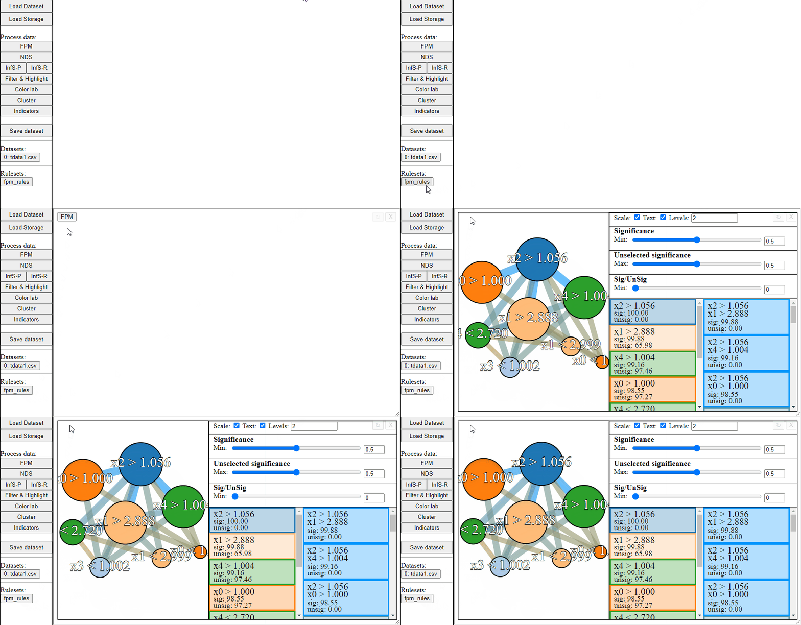
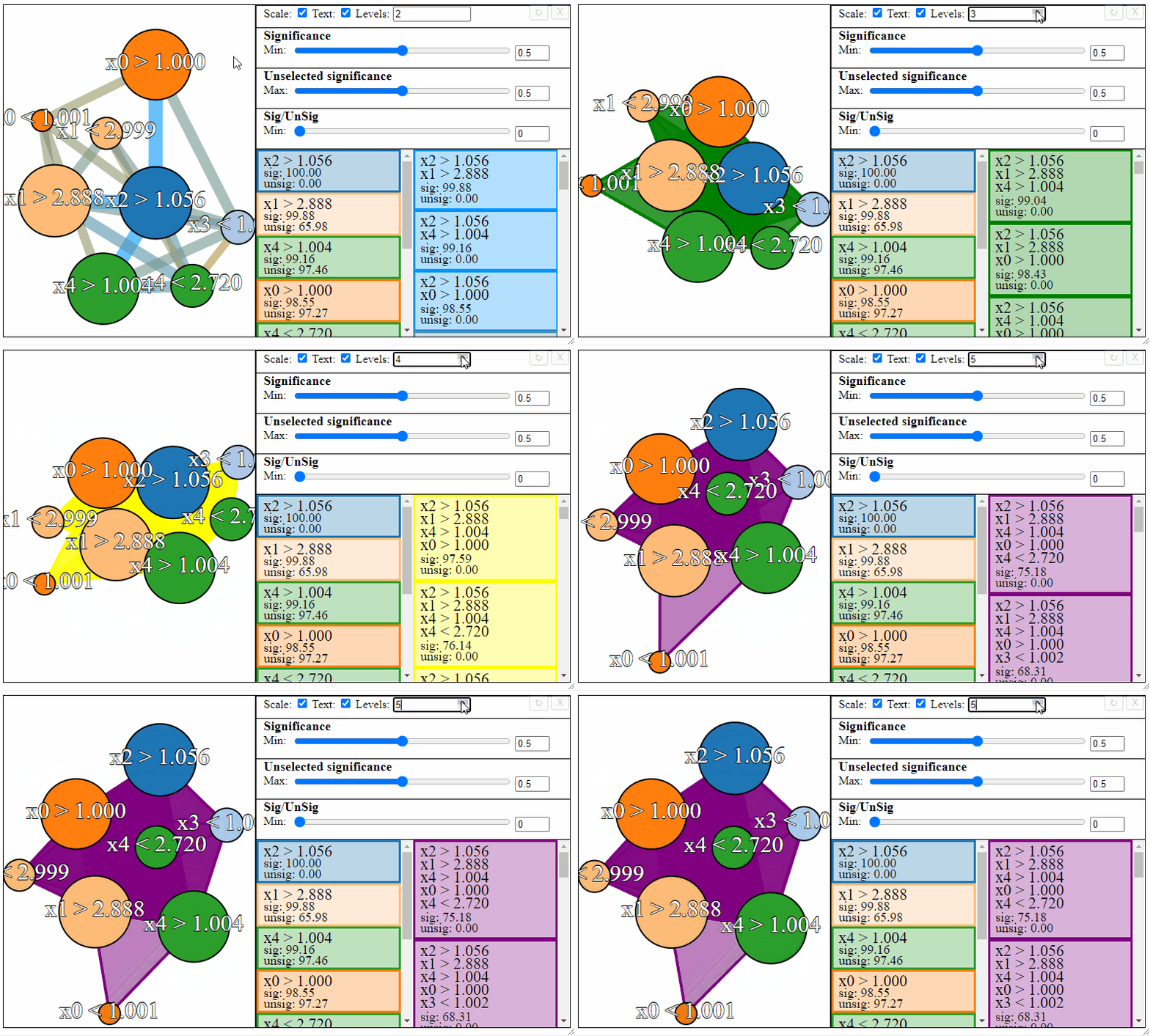
The nodes in the graph represent the individual FPM rules, and connections between the nodes represent rule-interactions. There are a number of parameters to modify to filter the graph:

1. Levels — The maximum desired levels of rule interaction
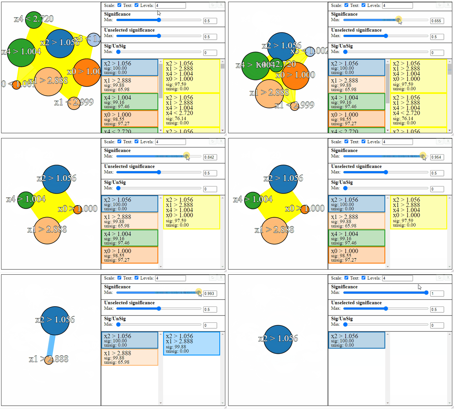
2. Significance — The minimum threshold significance of rules in the selected set
3. Unselected significance — The maximum threshold significance of rules in the unselected set
4. Sig/UnSig — The minimum threshold for significance ratio between the selected and unselected sets

Increasing the 'Levels' value will increase the allowed rule-interaction level, this corresponds to the 'Max. Levels' value set in the generation of the rules.

Rules can be filtered using the sliders to the right. Notice how the different slider give different results in the graph. The first slider limits the minimum allowed significance a rule or rule interaction may have, the second slider limits the maximum unselected significance a rule may have, and the third slider limits the ratio between the significance and the unselected significance that a rule may have.

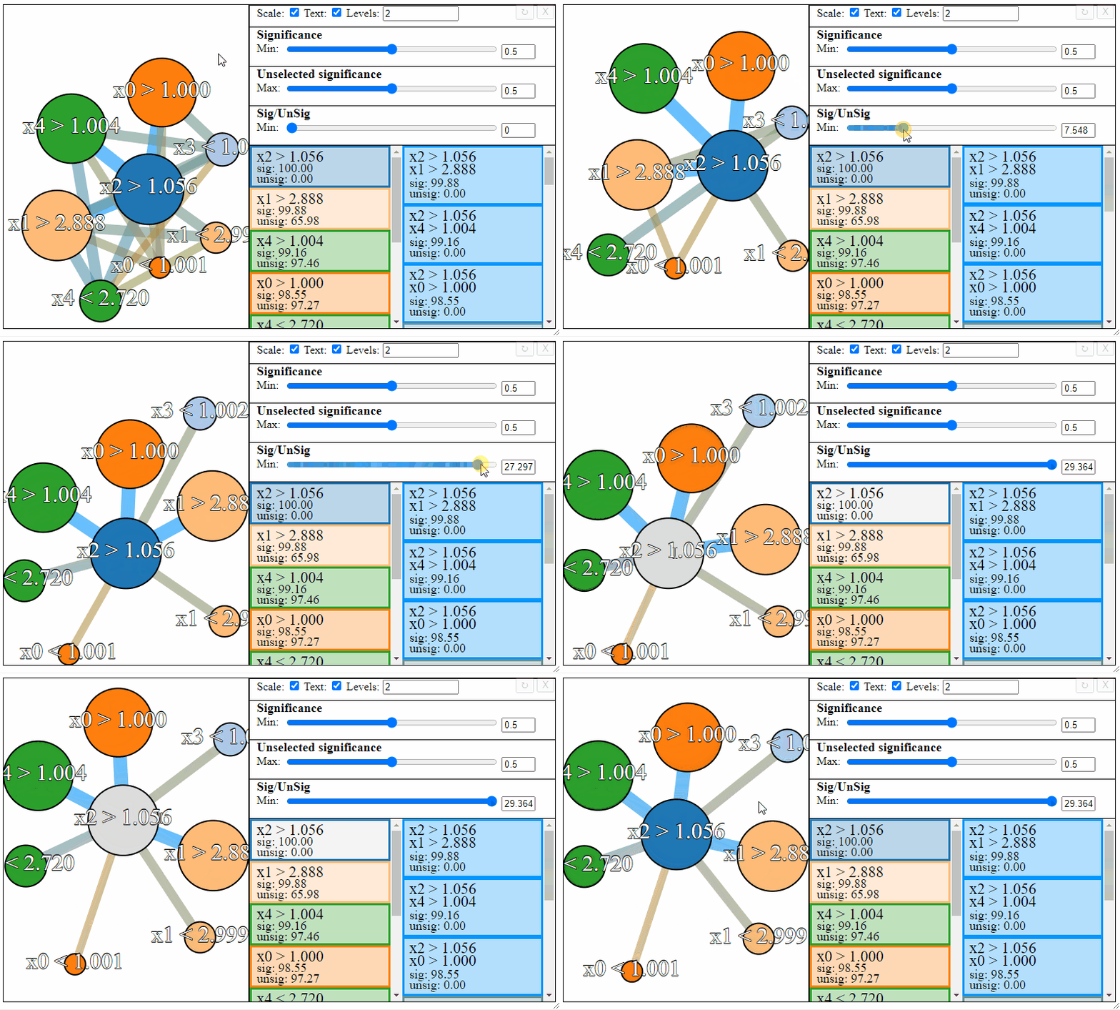
Different selections will result in different rulesets. Sometimes the most meaningful rules may require some trial and error to find.

Knowledge Validation

Once meaningful rules have been found using the graph interface, they can be validated by applying them as highlights in the original plot.
First right-click and copy the rule-interactions you have found.
Then open the 'Filter & Highlight' options pane and paste the rules into the text-box.
Finally, decide a color and click the highlight button to highlight the solutions that follow the rules.

References

[1] Tanabe, R. and Ishibuchi, H., 2020. An easy-to-use real-world multi-objective optimization problem suite. Applied Soft Computing, 89, p.106078.

[2] Hoffman, P., Grinstein, G., Marx, K., Grosse, I. and Stanley, E., 1997, October. DNA visual and analytic data mining. In Proceedings. Visualization'97 (Cat. No. 97CB36155) (pp. 437-441). IEEE.

[3] Van der Maaten, L. and Hinton, G., 2008. Visualizing data using t-SNE. Journal of machine learning research, 9(11).

[4] McInnes, L., Healy, J. and Melville, J., 2018. Umap: Uniform manifold approximation and projection for dimension reduction. arXiv preprint arXiv:1802.03426.

[5] Bandaru, S., Ng, A.H. and Deb, K., 2017. Data mining methods for knowledge discovery in multi-objective optimization: Part B-New developments and applications. Expert Systems with Applications, 70, pp.119-138.

[6] Dudas, C., Hg, A.H.C. and Bostron, H., 2009. Information extraction from solution set of simulation-Based multi-Objective optimisation using data mining. In 7th International Industrial Simulation Conference (pp. 65-69).